Sentiment Analysis using 1D Convolutional Neural Networks in Keras
“Quebec does not have opinions, but only sentiments” — Wilfrid Laurier

Note: I am a Machine Learning enthusiast interested in sharing what I have learned with others in the deep learning community with the hope that one might find some relevant information in it. I welcome all kinds of constructive criticism.
In this blog, we will discuss what Word Embedding, Tokenization, Callbacks, and 1D Convolutional Neural Networks are and how to implement a Sentiment Analysis model using the IMDB movie review dataset. For those in need of just the complete code, you can get it here.
Text Classification
It has become very necessary that maximum information is generated from data around us as data generation hit insane levels in the era. Data has become one of the driving forces behind many companies be it a small startup or large corporations. Unstructured data in the form of text is being generated everywhere: social media, chats, online and offline surveys, support tickets, social media and a lot more. There is absolutely no doubt that text is an extremely rich source of information, however, extracting insights from them can be very hard and time consuming due to its unstructured form.
Classifying textual content basically means assigning tags or categories to text according to its content. Although text classification is one of the fundamental tasks in Natural Language Processing, it has many broad and significant real life applications such as sentiment analysis, topic labelling, spam detection, intention detection, etc.

Businesses are relying on text classification for structuring text in a fast and cost-efficient way in order to boost profits by enhancing decision- making and also automating certain processes within their business pipelines.
There are quite a number of ways by which one can develop a text-classification system and in this post, we shall look at how Layered Representations Learning can be used to develop a sentiment analysis model to classify movie reviews from the popular IMDB dataset as either positive or negative. This model will be developed using 1D Convolutional layers.
1D Convolutional Layers
Convolutional Neural Networks (ConvNets) perform particularly well on computer vision problems due to their ability to operate convolutionally, that is extracting features from local input patches allowing for representation modularity and data efficiency. The same properties that make ConvNets the best choice for computer vision-related problems also make them highly significant to sequence processing. 1D convolution layers are also translation invariant in the sense that because the same input transformation is performed on every patch, a pattern learned at a certain position in a sentence can later be recognized at a different position. Similar to 2D ConvNets, 1D patches can be extracted from an input and output the maximum or average value, a process technically referred to as Max Pooling and Average Pooling respectively, and just as with 2D ConvNets, this is also used for reducing the length of the 1D input (technically known as subsampling).

Let’s now implement a basic 5-layered 1D ConvNet and use it to classify the IMDB movie reviews dataset as either positive or negative.
To begin, first download and uncompress the raw IMDB dataset from here. We will then retrieve the individual training reviews into a list of strings, one string per review and also collect the review labels into a list depicting a positive review as 1 and a negative as 0.
Afterwards, we tokenize our data. Tokenization is the act of breaking up a sequence of strings into smaller pieces such as words, keywords, phrases, symbols and other elements called Tokens. (Source: Techopedia). The text in each movie review is vectorized and the dataset is split accordingly into training and testing data after it has been shuffled.
The vectorized data can be decoded back to words using the following code.
Word Embeddings
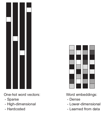
One powerful way to associate a word with a vector is by the use of dense word vectors, also known as word embeddings. Vectors obtained through one-hot encodings are mostly very sparse and very high-dimensional (same dimensionality as the number of words in the vocabulary). However, word embeddings are low dimensional floating-point vectors and unlike the vectors obtained from one-hot encoding, word embeddings are learned from the data at hand. In developing our model, we will use the Embedding layer in Keras to generate a 50 Dimensional word embedding from our dataset.

Building the Model

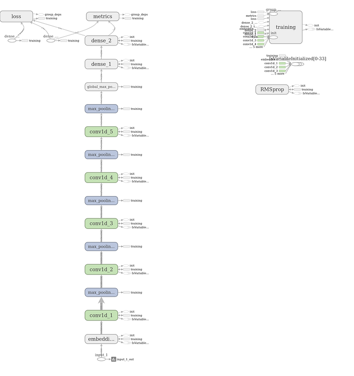
Finally, we build our model using Keras Functional API. The Keras Functional API gives us the flexibility needed to build graph-like models, share a layer across different inputs,and use the Keras models just like Python functions. As said earlier, this will be a 5-layered 1D ConvNet which is flattened at the end using the GlobalMaxPooling1D layer and fed to a Dense layer. Alternatively, the Flatten layer can also be used to accomplish this task. We then make our prediction by feeding the vector obtained from the Dense layer to another Dense layer of 1 unit and a sigmoid activation function. Our choice for a sigmoid activation function at the output layer is because our classification task involves only two classes (either positive or negative). The code for building the model is pasted below:
Also shown in the figure below is the accompanying graph of the model generated using TensorBoard.

With the model ready for use, we will now go ahead and fit it to the training and validation data using the following code:
Callbacks

We tend to lose control over how our model trains on the provided dataset the moment we call the fit() or fit_generator() method on our model and this means that with a model not “smart” enough, we can only watch it perform very badly during training or quit the training and start allover again. This process can really be expensive and ineffective therefore in order to avoid that, we would like to develop a model that can self-introspect and dynamically take action that will positively affect training. There are many things one cannot predict during training. For instance, one cannot tell the exact number of epochs that will be needed to achieve an optimal validation loss and accuracy.

Mostly during training, we tend to use an arbitrary number of epochs and if the model overfits before that number of epochs is reached then we reduce the number of epochs and train again otherwise, we increase the number of epochs and this approach is very wasteful. A much better way to handle this during training is to stop training when we realize that the validation loss is no longer improving. This can be achieved using a Keras callback. A callback is an object (a class instance implementing specific methods) that is passed to the model in the call to fit and that is called by the model at various points during training. It has access to all the available data about the state of the model and its performance, and it can take action: interrupt training, save a model, load a different weight set, or otherwise alter the state of the model.
Some ways by which callbacks can be used are:
- Model checkpointing — Saving the current weights of the model at different points during training.
- Early stopping — Interrupting training when the validation loss is no longer improving (and save the best model obtained during training).
- Dynamically adjusting the value of certain parameters during training such as the learning rate optimizer.
- Logging training and validation metrics during training or visualizing representations learned by the model as they’re updated. (The Keras progress bar we always see in our terminal during training!)
A snippet how to implement callbacks in Keras is shown below:
Callbacks are passed to the during via the callback argument in the fit() method which takes a list of callbacks. Any number of callbacks can be passed to it.
The monitor argument in the EarlyStopping callback monitor’s the model’s validation accuracy and the patience argument interrupts training when the parameter passed to the monitor argument stops improving for more than the number (of epochs) passed to it (in this case 1).
The filepath argument in the ModelCheckpoint callback saves the current weights after every epoch to the destination model file and the monitor and save_best_only arguments mean we won’t override the model file unless the validation loss (val_loss) has improved. This allows us to keep the best model seen during training.
Also, the ReduceLROnPlateau callback is used to reduce the learning rate when the validation loss has stopped improving. This has proven to be a very effective strategy to get out of local minima during training. The factor argument takes as input a float which is used to divide the learning rate when triggered.
Tensorboard

The key purpose of TensorBoard is to help us visually monitor everything that goes on inside our model during training. Tensorboard gives us access to several relevant features such as
- visually monitoring metrics during training
- visualizing the architecture of our model
- visualizing histograms of activations and gradients
- exploring embeddings in 3D
Berefore using tensorboard, we will need to first create a directory where the log files it generates will be stored using the following command on the command line.
$ mkdir log_dir_m1(to create the log_dir_m1 directory in this case). TensorBoard can be launched as part of our callbacks and it takes as parameters the location where the log files will be written, and the frequency (in epochs) at which the activation histograms and embeddings will be recorded.
At this point, we can launch the TensorBoard server from the command line, instructing it to read the logs the callback is currently writing. Tensorboard is automatically installed with Tensorflow and it can be started with the command below on the command line.
$ tensorboard --logdir=log_dir_m1With the server started, we can then browse to http://localhost:6006 and look at the model training. In addition to the training and validation metrics,

We can also access the Activation and Gradient Histogram Tabs where we can obtain neat and pretty visualizations of activation values taken by our layers such as the example shown below.

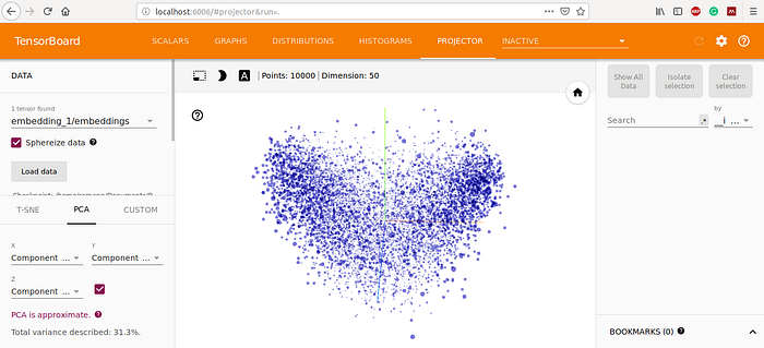
TensorBoard also generates the graphical architecture of our model. The embedding tab also gives us a way to inspect the embedding locations and spatial relationships of the 10,000 words in the input vocabulary as learned by the embedding layer but because the embedding space is 50-Dimensional, TensorBoard automatically reduces it to 2D Or 3D using dimensionality-reduction algorithms such as Principal Component Analysis (PCA) or T-distributed Stochastic Neighbor Embedding (t-SNE). In the point cloud in the figure below, we can clearly see two clusters denoting words with a positive connotation and words with a negative connotation. This shows that the embeddings in our model trained with the specifically to the task at hand (that is classifying the movie ratings) and this is one of the major reasons it is advisable to train a word embedding based on a specific task instead of using pretrained generic word embeddings. (I found this in-depth tutorial of TensorBoard very helpful and you might want to check it out for a deeper dive into TensorBoard.)

Making Predictions

We will now go ahead and test our model after evaluating it on our test data. We will also go an extra mile to score text fed to our system in different ways. The complete codes for this project can be accessed here.
Loading the Model and Tokenizer

During our data preprocessing, we used the Tokenizer in Keras on our dataset to convert it from text to sequences before padding it to ensure consistency in input to our layer. During scoring of test data, it would be just logical that we use the same tokenizer that we used on our training data on the test data as well. In order to achieve this, we would have to save the tokenizer that was fit on the training data as a pickle object. Therefore after tokenizing the training data in Part 1, we use the following code to save the tokenizer as a pickle object.
Also, during training, we were able to save the best model obtained as “movie_sentiment_m1.h5” in a directory called model. We will therefore load the model using the load_model method in the Keras models class and also load the tokenizer which was saved as a pickle object using the load method in the pickle module. The process described above can be achieved using the code in the snippet below.
With our model and tokenizer at hand, we will then go ahead and write a simple script to score our text samples (found in the test_dir folder in github repository).
Scoring the Text Samples

Although scoring the text samples is pretty straight forward, we would like to write a simple script which will enable us accept text content as a simple string data, a list of strings, a file containing the text to be scored, and a directory containing a number of text files with texts to be scored in them.
In addition to that, we would also like to display not only the score of the review but also a scale showing the polarity of the score accompanied with the actual review that was scored.
To begin with, we will first write a simple method which accepts as arguments the score of the review and the review that was scored and based on the score, a polarity scale from ranging “Strongly Positive” down to “Negative” is assigned to the score and the output is printed out.
We then write another method to decode the review (similar to what was done in Part 1). This method takes as input a list of string objects (containing the text) which gets converted to sequences using our tokenizer and then padded to match the input length that was used for the model during training. This method then returns the decoded review and the padded sequence.
Finally, we add the last method which will accept the data in various formats. This method will take the source of the text and the type of file (if its a file or a directory of files) as arguments. We then process them according to the source. Basically, with a source as a simple string, we append that to a list and feed this list to the decoded review method which returns the sequence in its padded form and the decoded review. We then call the predict() method on the model and pass the padded sequence returned to it to obtain the score. With the score and the decoded review, we pass these information to the review_rating method to obtain the a pretty output to be displayed. Data from other sources (directory of files of a list of string texts) basically go through similar processes, in for loops.
We can then go ahead and test the score review method by using sample data available in the test_dir repository using the following code:
score_review('test_dir/test', file_type='dir')A sample output obtained from testing the review samples in file formats inside the test directory (found in the test_dir folder in the github repository) is displayed in the image below.


Conclusion

In this post, we were able to understand the basics of word embedding, tokenization, and 1D Convolutional Neural Network and why it is suitable for Text Classification and Sequence processing. We also learned about the concept of callbacks, its importance and how to implement it in the Keras framework. We successfully tested our model on test data from different fanciful sources. Finally, we saw how to build a Layered Representational Network using Functional APIs in Keras. I hope we all enjoyed ourselves on these project and learned a ton of good stuffs along the way. Have a nice day!

I am very grateful to Francois Chollet for his book on Deep Learning and Steven Bird, Ewan Klein, and Edward Loper for their book on Natural Language Processing. I also thankful to Andrew Trask for his tweet which encouraged the writing of any new information or knowledge obtained since it is only by explaining what you have learned that you can know what you have really learned.
Check out this article for a deeper dive into Tensorboard: https://bit.ly/2STa5Ax
